West Nile Virus (WNV) Prediction with Classical Machine Learning

In this page, I walk through my approach to predicting West Nile Virus (WNV) cases in California counties from 2004 to 2023 using Support Vector Regression (SVR), Random Forest (RF), and Histogram Gradient Boosting Regressor (HGBR).

The process involves key steps such as data preparation, hyperparameter tuning, model training, and performance evaluation. I also explore advanced techniques like bootstrapping to assess model reliability and SHAP-based feature interpretation to uncover the drivers behind the predictions.

1. Data Preprocessing

Steps

• Load data and remove unnecessary columns.
• Drop zero-variance features and handle missing values
• Data between year 2004 and 2018 are selected as training data, after 2018 as testing data
• 80% of the training data are used for hyperparameter tuning, the other 20% are used for validation
• Normalize features using StandardScaler

2. Support Vector Machine (SVM)

Optimize the hyperparameters of the Support Vector Regression (SVR) model using hyperopt to improve predictive accuracy.

Steps

• Define a search space for SVM hyperparameters (C, epsilon, kernel, and gamma).
• Use the hyperopt library to perform the search.
• Train the final model using the best hyperparameters.

3. Random Forest (RF)

Optimize the hyperparameters of the Random Forest Regressor (RF) model to improve predictive accuracy.

Steps

• Define the hyperparameter search space (n_estimators, max_depth, min_samples_split, min_samples_leaf, etc.).
• Use the hyperopt library to find the best combination of hyperparameters.
• Train the final model with the selected hyperparameters.

4. Histogram-based GradientBoostingRegressor (HGBR)

Optimize the hyperparameters of the HistGradientBoostingRegressor (HGBR) model for accurate WNV predictions.

Steps

• Define the hyperparameter search space, including parameters like max_depth, learning_rate, and max_iter.
• Use the hyperopt library to perform optimization.
• Train the final model with the selected hyperparameters.

5. Model Comparison

Compare the performance of the three models—SVM, Random Forest (RF), and HistGradientBoostingRegressor (HGBR)—using Q² and Mean Squared Error (MSE) metrics.

Steps

• Collect R² and MSE metrics for each model.
• Visualize the results to compare performance.

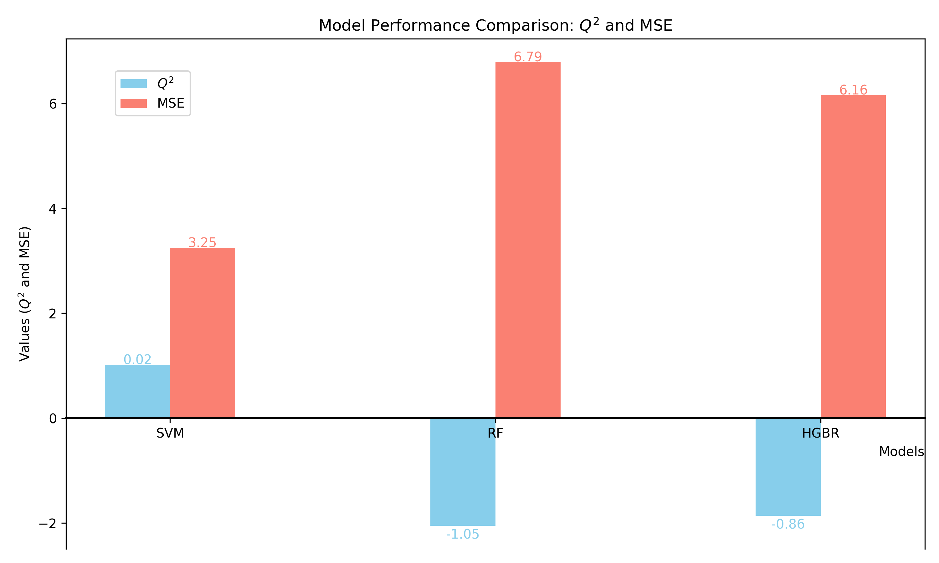
Figure 1: Model evaluation with Q² and MSE, Red represents Q² and blue represents MSE

6. Bootstrapping for Robust Estimation

Additionally, incorporating bootstrapping to estimate 95% confidence intervals ensures a robust understanding of SVM model performance, offering insights into the variability and reliability of the results. This rigorous approach supports confident decision-making in modeling and prediction.

Steps

• Bootstrapping using test data from 2019 to 2023
• Based on the model trained on training data from 2004 to 2018
• Perform bootstraping with 1000 iteration, store the Q² and MSE value for each iteration
• Calcultae 95% confident interval
• Plot the bootstrapping results

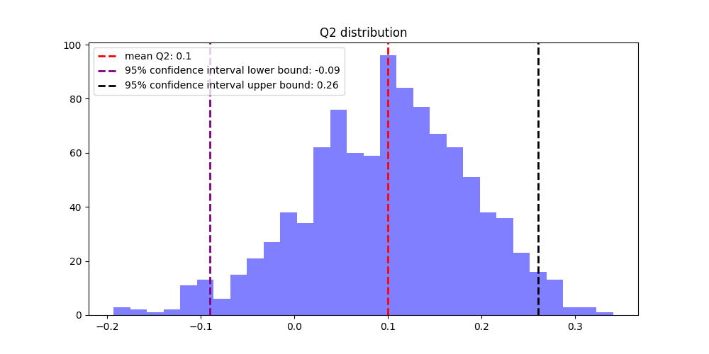
Figure 2: Bootstrapping result of Q² distrbution, itr=1000

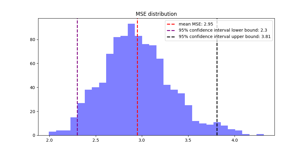
Figure 3: Bootstrapping result of MSE distrbution, itr=1000

7. SHAP Value Analysis for Variable Importance

Analyze the predictions of the SVM model using SHAP values to identify the contribution of each feature to the model's output.

Figure 4: Bar plot of Global SHAP values to overall variable importance. The mean absolute value of each feature over all the instances (rows) of the dataset as global SHAP value

In order to check how each individual sample contribute to the model's prediction, you can specify Year, Month and County to see specific sample and what is each variable's contribution to the prediction of this sample.

Figure 5: Bar plot of Local SHAP value to show individual sample variable importance