Population genetics of Culex tarsalis

Individual mosquitoes were trapped and collected from 28 different locations across the United States and Canada as part of the North American Mosquito Project (NAMP) (Cohnstaedt et al. 2016). All samples used in this study were collected in 2012 between the months of April and October.

1. ADMIXTURE and PCA

The ADMIXTURE analysis indicated a strong signature of population structure among the collected samples, with the optimal number of population assignments occurring at K=4 (Figure 2C). The genetic clusters corresponded to four different broad geographic regions: (1) California/the West Coast, (2) the Southwest, (3) the Northwest, and (4) the Midwest (Figure 1).

The PCA results confirmed this pattern, while also showing evidence of some sub-structure among the West Coast and Northwest populations (Figure 2C). Voronoi Tessellation Plot (Figure 3) also Reveals a East-West Spatial Genetic Gradient.

**Figure 2: Population Structure of Cx. tarsalis result using ADMIXTURE and PCA** (A) Floating pie charts of the admixture proportions in Cx. tarsalis populations sampled across the Western and Midwestern U.S and parts of Canada. Pie chart sizes are proportional to the sample size at each collection site. (B) ADMIXTURE results for K=4. Labels along the x-axis indicate sampling locations and colors correspond to the admixture proportion for each of the 4 clusters. (C) PCA results for the top 2 principal components, with points colored by the 4 geographic regions identified by ADMIXTURE.

**Figure 3: Spatial Distribution of Genetic Variation and Sampling Locations** Polygons/cells represent regions of influence for each sampling location, filled with a gradient from light green (low PC1 mean scores) to dark green (high PC1 mean scores), highlighting spatial genetic variation. Points represent sampling locations, colored by assigned regions (West Coast, Northwest, Midwest, Southwest), grouping populations geographically.

2. Analysis of MOlecular VAriance (AMOVA)

An Analysis of MOlecular VAriance (AMOVA) was performed using the poppr package's poppr.amova() function in R to detect population differentiation among regions inferred from ADMIXTURE results. To assess whether there was a statistically significant level of population structure, a randomization test was conducted using the randtest() function from the ade4 package in R, employing 999 replicates.

**Figure 4: AMOVA significant test results** Gray bars indicate the expected distributions based on 999 random permutations, while black bars indicate the observed phi values. (A) Variation within populations, (B) Variation between populations within the same region, and (C) Variation between different regions.

3. Isolation by Distance (IBD) verse Isolation by Environment (IBE)

Both geographic distance (IBD) and environmental distance (IBE) were tested for their relationships with genetic distance. The Mantel test revealed a strong and statistically significant correlation between genetic and geographic distances, with a Mantel statistic of 0.5661 (p < 0.001), indicating that geographic distance plays a notable role in genetic differentiation in this system. In contrast, the relationship between genetic and environmental distances was weak and non-significant, with a Mantel statistic of -0.05185 (p = 0.7741).

**Figure 5: Isolation-by-Distance and Isolation-by-Environment** (A) Pairwise geographic distance versus genetic distance (FST) with best fit linear regression model (red line: y = 0.012+8.4×10^(-8) x,R^2=0.3). (B) Pairwise environmental distance versus genetic distance with best-fit linear regression mode (red line: y=0.06+0.021x0.14-0.0025,R^2=0.040.0014). (C)Kernel density plot with best fit spline for geographic distance versus genetic distance. Areas of high, intermediate, and low density are represented by red, yellow, and blue colors, respectively. (D) Kernel density plot with best-fit spline for environmental distance versus genetic distance. Each point in panels A, B, C, and D represents one individual sample.

4. Partial Redundancy Analysis (Partial RDA)

To further investigate the potential role of environmental factors, we performed partial redundancy analysis (partial-RDA) to separate and evaluate the individual contributions of geographic (IBD) and environmental (IBE) factors to genetic differentiation.

Table 1: Key Statistical Outputs of Partial RDA Analysis
Model	R² (Adjusted)	F-statistic	p-value
Environment (Controlling for Geography)	0.0309	2.36	0.001***
Geography (Controlling for Environment)	0.0134	3.32	0.001***

Significant Code: 0 ‘***’ 0.001 ‘**’ 0.01 ‘*’ 0.05 ‘.’ 0.1 ‘ ’ 1

Table 2: Redundancy Analysis (RDA) Biplot Scores for Constraining Variables
Variable	RDA1	RDA2	RDA3	RDA4	RDA5	RDA6
eastward_wind	-0.04295	0.6138	-0.38221	-0.068225	0.2848	0.4225
northward_wind	-0.01733	-0.1283	-0.60759	0.469732	-0.1585	-0.2478
temperature	0.25899	-0.2221	-0.03984	0.016740	0.1733	-0.1052
high_vegetation	0.07189	0.4416	0.11040	0.411215	0.4095	-0.3103
low_vegetation	-0.78515	-0.3226	0.03450	-0.004408	0.1817	-0.2035
water_retention_capacity	-0.50671	-0.2401	0.33451	0.665514	0.0183	0.1856
surface_runoff	-0.37392	-0.4824	0.22363	0.196856	0.3530	0.2560
evaporation	0.56079	0.3324	-0.01991	-0.094839	-0.2216	0.1812

5. Genotype-Environmental associatioins (GEA) using Redundency Analysis (RDA)

The RDA operates as a multifaceted ordination technique, evaluating multiple loci concurrently with environmental variables. For this analysis, the significance of both the overall RDA model and its individual constrained axes was assessed. This assessment utilized the anova.cca() function from the vegan package in R (Oksanen et al. 2019; Borcard et al.), facilitating a comprehensive examination of the null hypothesis (an absence of a linear relationship between SNP data and environmental variables). To select candidate SNPs for local adaptation, we identified SNPs that significantly deviated from the mean loadings, using a threshold of 3 standard deviations. Statistical significance was determined based on p-values below the threshold of 0.001.

**Table 3: Significant test results on each constrained axis of RDA**
	Df	Variance	Proportion	F	Pr(>F)	Significance
Full Model	8	1796.3	10.42%	4.5511	0.001	***
RDA1	1	894.1	5.19%	18.1217	0.001	***
RDA2	1	469.8	2.73%	9.5231	0.001	***
RDA3	1	158.7	0.92%	3.2158	0.001	***
RDA4	1	69.8	0.40%	1.4154	0.001	***
RDA5	1	56.8	0.33%	1.1517	0.094	.
RDA6	1	51.1	0.30%	1.0361	0.591
RDA7	1	48.6	0.28%	0.9855	0.901
RDA8	1	47.3	0.27%	0.9592	0.901
Constrained axis Residual	313	15442.7

Significant Code: 0 ‘***’ 0.001 ‘**’ 0.01 ‘*’ 0.05 ‘.’ 0.1 ‘ ’ 1

**Figure 6: Environmental Correlates of Genetic Variation in Cx. tarsalis Across Diverse North American Regions.** Panels A and B display the relationship between environmental factors and the distribution of Cx. tarsalis, using RDA to illustrate how regional differences affect genetic variation. In these panels, the position of each circle (representing an individual mosquito) and color (indicating regional groupings from ADMIXTURE results) reflects their association with environmental variables, shown as purple vectors. The first plot (A) focuses on RDA1 and RDA2, the primary axes explaining the most variance, while the second (B) explores more subtle influences in RDA3 and RDA4.

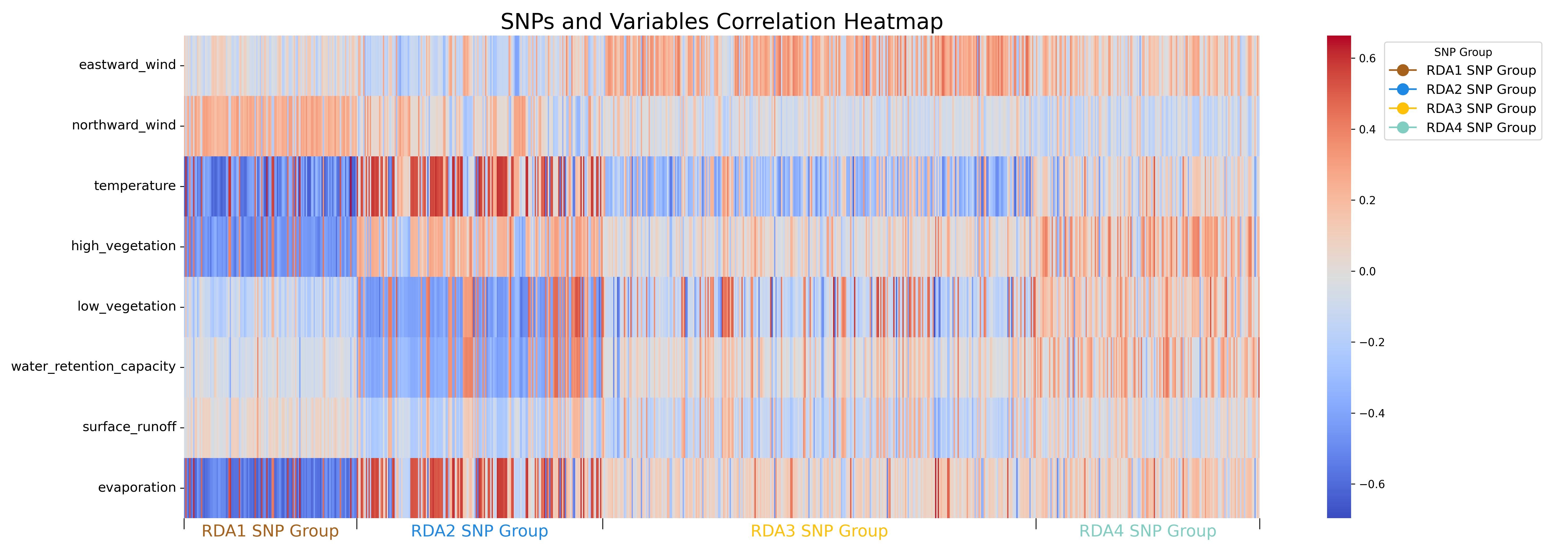
**Figure 7. Correlation Heatmap between Environmental Variables and RDA Candidate SNPs.** This heatmap illustrates the correlation between the environmental variables and candidate SNPs identified through the first four constrained axes of Redundancy Analysis (RDA). Each column on the x-axis represents a candidate SNP. For detailed SNP names and associated information on the 17 genes identified by SIFT4G, please refer to Supplemental Figure 3.

6. SNPs Under Selection

To find which SNPs that were significantly associated with environmental variables also showed signatures of natural selection, we performed a Bayesian selection inference as implemented in BayeScan. We also independently identified outliers using a PCA-based method implemented in the pcadapt R package

**Figure 8: BayeScan results**

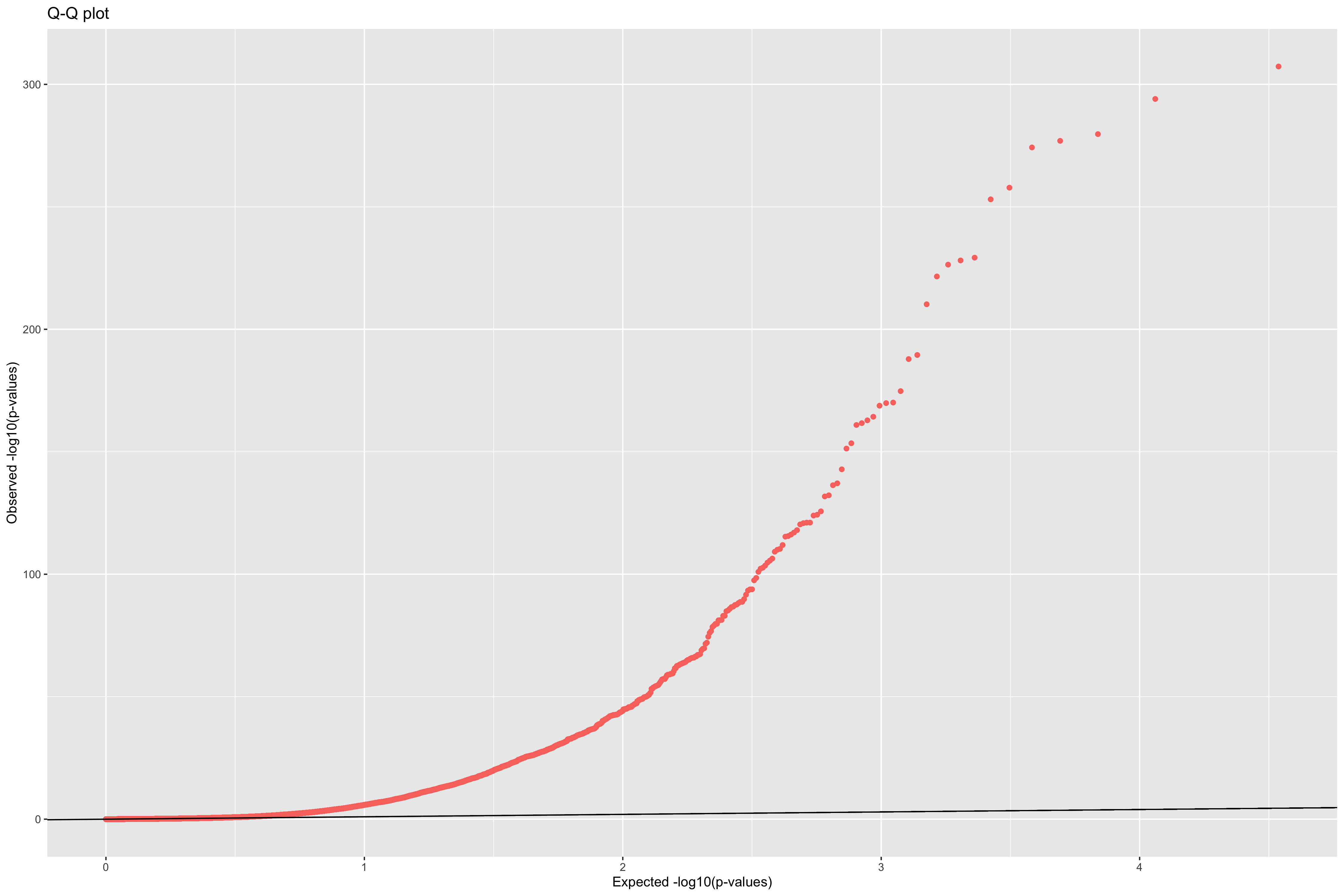
**Figure 9: Q-Q plot to check the expected uniform distribution of the p-values in PCAdapt.**

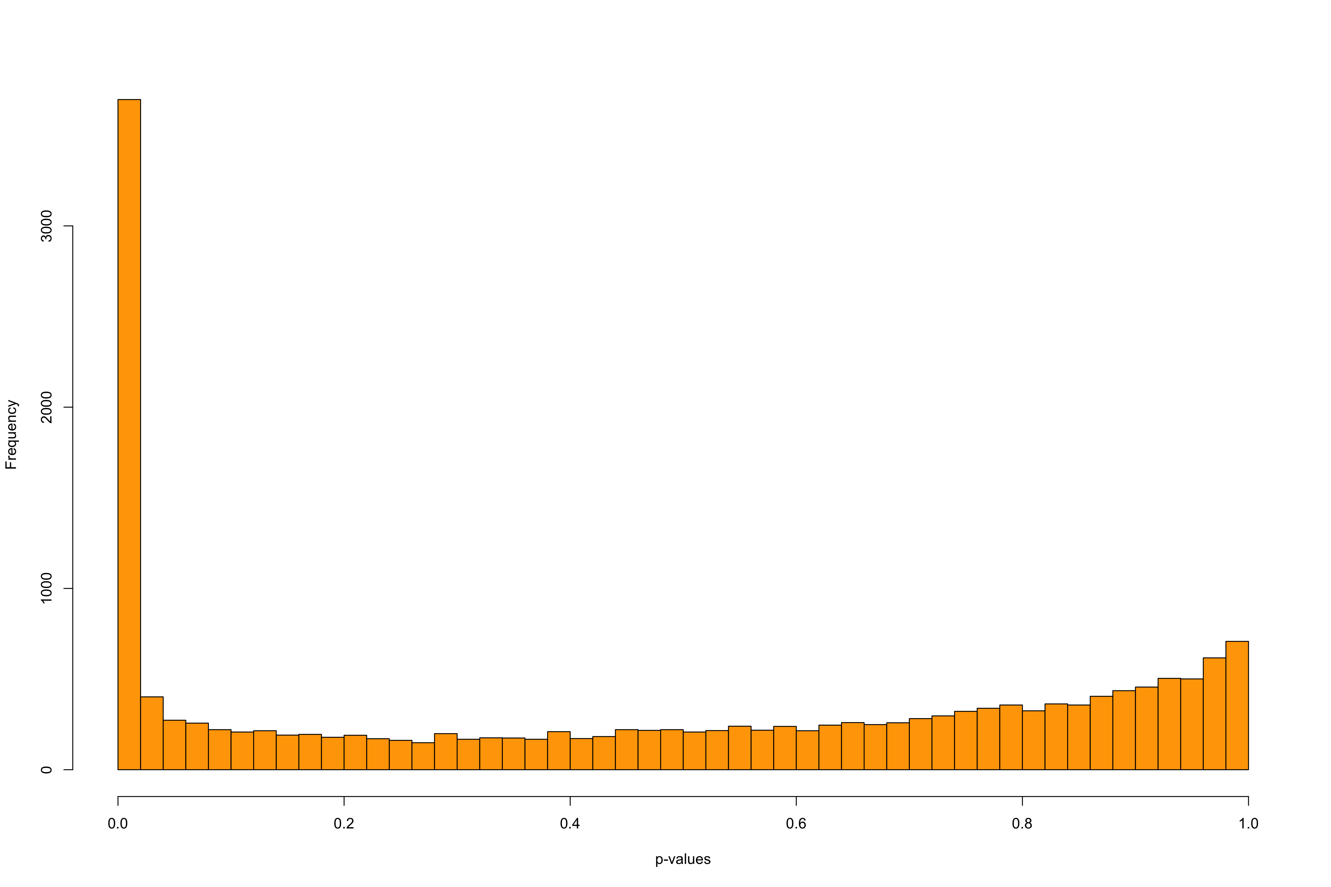
**Figure 10: Histograms of the test statistic and of the p-values in PCAdapt** Most of the p-values follow an uniform distribution. The excess of small p-values indicates the presence of outliers.

7. Overlapping Candidate Adaptive Genes

Looking across all four analyses examining significant environmental associations and evidence of natural selection, we identified 20 common genes containing candidate SNPs that were consistently significant in each instance. Given BayeScan’s susceptibility to potential false positives, we included PCAdapt to provide additional validation and strengthen the robustness of our findings.

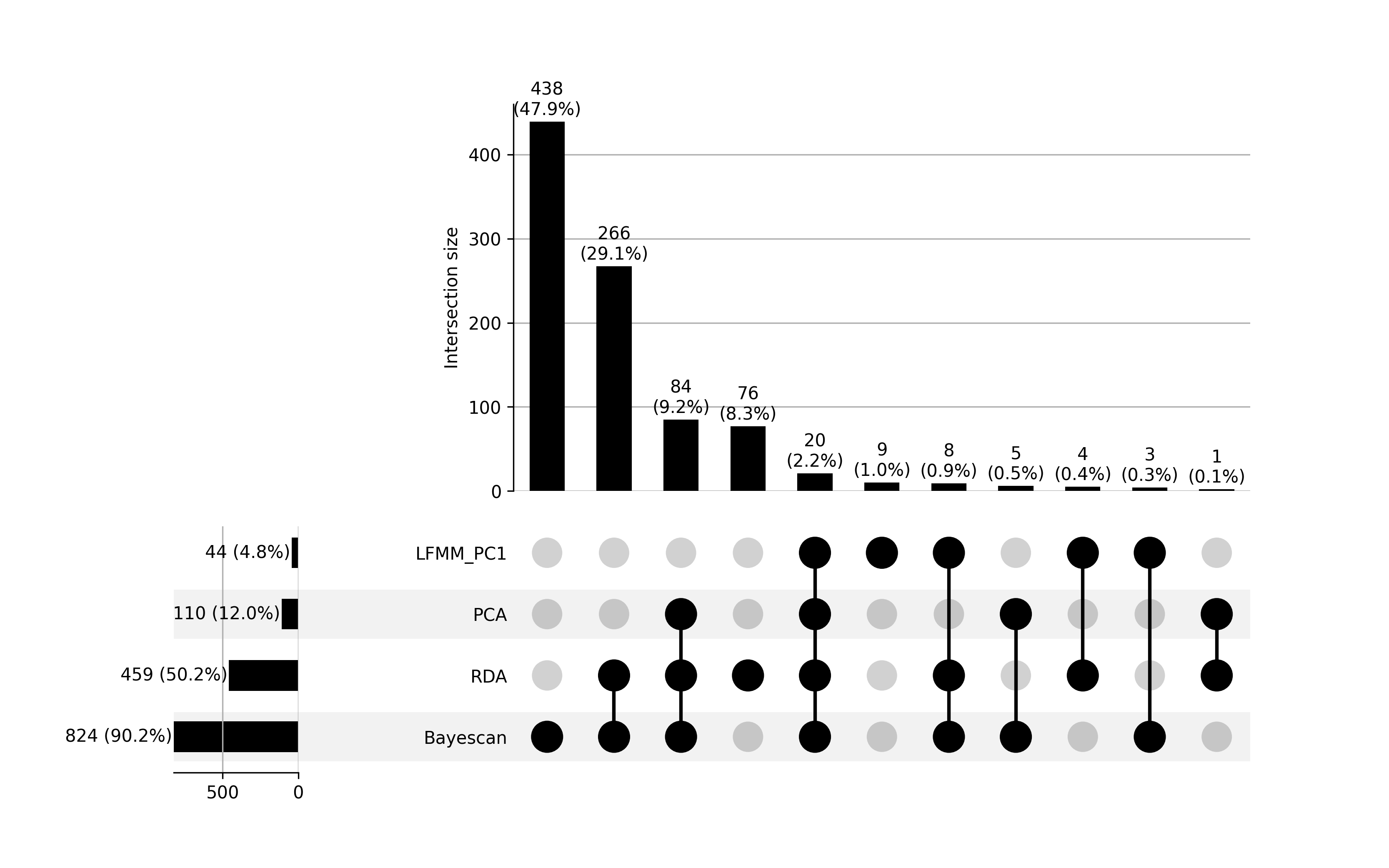
**Figure 11: Upset Plot showing the overlap of genes annotated from candidate SNPs identified across four methods for detecting local adaptation and environmental associations in Cx. tarsalis: LFMM, RDA, PCAdapt, and BayeScan.** The bar heights indicate the number of genes annotated based on candidate SNPs in each unique or shared category, with percentages relative to the total genes annotated. Black circles below the bars represent intersections of methods, where connected lines indicate the methods contributing to the overlap. For example, the tallest bar corresponds to 438 genes uniquely identified by BayeScan (47.9%), with no overlap with other methods. Individual horizontal bars represent the total number of genes identified by each method: LFMM_PC1 (44, 4.8%), PCA (110, 12.0%), RDA (459, 50.2%), and BayeScan (824, 90.2%).